You have a €5,000 Bankroll.
Your usual rule is simple:
1U = €50, representing 1% of your Bankroll.
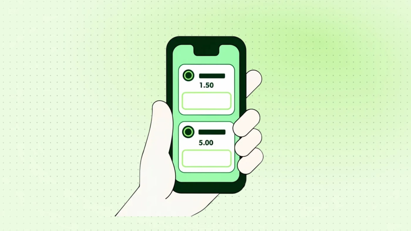
Two sports betting opportunities become available.
The first offers odds of:
1.50 (-200)
The second offers odds of:
5.00 (+400)
Should you stake €50 on each selection?
Or should you bet more at 1.50 (-200), because the outcome is considered more likely, and less at 5.00 (+400), because the outcome is considered riskier?
The answer is less obvious than it might seem.
Low odds do not necessarily mean that a bet offers good value.
High odds do not necessarily mean that a bet is a bad opportunity.
Most importantly:
Odds alone are not enough to determine the optimal Stake.
To understand why, we need to distinguish three fundamental concepts:
- The probability of winning.
- The Expected Value of the bet.
- The financial risk associated with the Stake.
1. What Do Betting Odds Actually Represent?
Decimal odds indicate the total amount returned when a bet wins, including the original Stake.
American Odds express the same potential return using positive or negative numbers.
Negative American Odds indicate how much you must stake to earn 100 units of profit.
Positive American Odds indicate how much profit you earn from a 100-unit Stake.
For example, with a €50 Stake:
At 1.50 (-200), the total return is €75, including €25 in net profit.
At 5.00 (+400), the total return is €250, including €200 in net profit.

However, potential profit is only one part of the equation.
You must also consider the probability of winning.
2. The Implied Probability of Betting Odds
Every set of betting odds corresponds to an implied probability.
For decimal odds, the formula is:
Implied Probability = 1 / Decimal Odds × 100
For American Odds, the equivalent formulas are:
For negative odds:
Implied Probability = |American Odds| / (|American Odds| + 100) × 100
For positive odds:
Implied Probability = 100 / (American Odds + 100) × 100
Here are several examples.
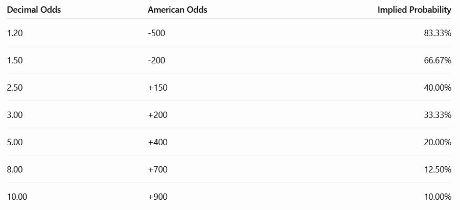
These implied probabilities represent the break-even thresholds associated with the quoted odds.
They do not necessarily represent the true probabilities of the outcomes.
In particular, bookmaker odds generally incorporate a margin.
To identify a valuable betting opportunity, you must compare the implied probability with your own estimate of the true probability.
3. Is a Bet at 1.50 (-200) Necessarily Less Risky Than One at 5.00 (+400)?
In terms of winning frequency, a selection priced at 1.50 (-200) is generally expected to win more often than a selection priced at 5.00 (+400).
However, this does not automatically make it more profitable.
Let's consider two bets.
Bet A: 1.50 (-200)
Estimated true probability:
70%
Implied probability:
66.67%
The estimated probability is higher than the break-even threshold.
Therefore, this bet has a positive Edge, assuming your probability estimate is correct.
Bet B: 5.00 (+400)
Estimated true probability:
25%
Implied probability:
20%
Once again, the estimated probability exceeds the break-even threshold.
This second bet also has a positive Edge.
However, the two bets have very different risk profiles.
4. Expected Value Allows Us to Compare Both Bets
Expected Value, or EV, measures the theoretical average profit or loss from a bet over a very large number of repetitions.
Using decimal odds, the expected ROI formula is:
EV (%) = (True Probability × Decimal Odds - 1) × 100
Bet A: 1.50 (-200)
Estimated probability:
70%
Calculation:
(0.70 × 1.50 - 1) × 100 = +5%
Expected Value:
+5%
Bet B: 5.00 (+400)
Estimated probability:
25%
Calculation:
(0.25 × 5.00 - 1) × 100 = +25%
Expected Value:
+25%
The bet at 5.00 (+400) has a significantly higher Expected Value in this example.
However, that does not automatically mean you should stake more on it.
Why?
Because its results are much more volatile.
5. Higher Odds Generally Mean Greater Variance
At odds of 1.50 (-200), a selection can win relatively frequently.
At odds of 5.00 (+400), even an excellent selection may lose three times out of four.
This means losing streaks can be considerably longer.
Let's compare our two bets.
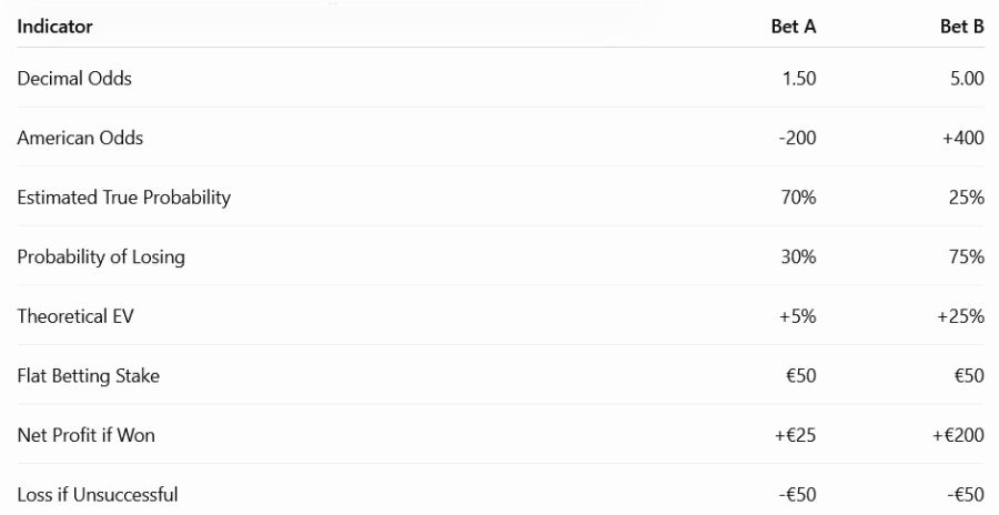
With an identical Stake, the maximum loss on each individual bet remains €50.
However, the frequency and distribution of wins are very different.
6. Losing Streaks: The Difference Between 1.50 (-200) and 5.00 (+400)
Let's assume that our estimated true probabilities are correct and that the events are independent.
For the bet at 1.50 (-200), the probability of losing is 30%.
For the bet at 5.00 (+400), it is 75%.
We can calculate the probability of losing several consecutive bets.

These percentages apply to one specific sequence of independent bets, not to the probability of experiencing at least one such streak during an entire season.
Nevertheless, the conclusion is particularly important:
A strategy targeting high odds can experience long periods without a win while maintaining a positive Expected Value.
This is why Bankroll Management cannot be based on ROI alone.
7. A Profitable Strategy at 5.00 (+400) Can Be Psychologically Difficult to Follow
Imagine a Strategy with the following characteristics:
Average Odds:
5.00 (+400)
True Win Rate:
25%
Theoretical EV:
+25%
Over 100 bets, the theoretical expected number of wins is 25.
However, this does not mean you will win exactly one out of every four bets.
You may experience:
- Several wins close together.
- Ten bets without a single win.
- An extended losing period.
- A few subsequent wins that compensate for earlier losses.
Long-term ROI may be attractive.
But Variance can be substantial.
Such a strategy therefore requires an appropriate Bankroll and considerable discipline.
8. Flat Betting: Should You Use 1U Regardless of the Odds?
Flat Betting means staking the same Unit on every selection.
In our example:
Bankroll = €5,000
1U = €50
You stake:
€50 at 1.50 (-200)
and:
€50 at 5.00 (+400)
This approach offers several advantages.
It allows you to:
- Limit the maximum loss on each bet to one Unit.
- Avoid emotional decisions.
- Compare strategy performance on a consistent basis.
- Track results easily in Units.
- Reduce Stake Sizing errors.
However, Flat Betting does not mean that every strategy carries the same level of risk.
A Strategy consisting mainly of bets at 5.00 (+400) may experience larger Drawdowns than one consisting mainly of bets at 1.50 (-200), even if both use 1U per bet.
9. Flat Betting Is a Risk Management Rule, Not an Optimization Method
We need to distinguish two objectives.
Objective 1: Control Risk Simply
Flat Betting is particularly suitable.
You decide that one Unit represents 1% of your Bankroll.
Each bet therefore has a clearly defined financial exposure.
Objective 2: Optimize Theoretical Bankroll Growth
It may be appropriate to adjust Stakes according to the Edge and risk of each opportunity.
This is one of the objectives of the Kelly Criterion.
However, such optimization requires reliable estimates of true probabilities.
And that is precisely the main difficulty.
10. Why Betting More at 1.50 (-200) Is Not Automatically a Good Idea
A common mistake is thinking:
"The odds of 1.50 (-200) are safer, so I can bet twice as much."
Suppose you stake:
€100 at 1.50 (-200)
and:
€50 at 5.00 (+400)
If the bets lose:
The bet at 1.50 (-200) costs you €100.
The bet at 5.00 (+400) costs you €50.
You have doubled your financial risk on the selection considered more likely to win.
However, a higher probability of winning does not guarantee a better Expected Value.
Consider this example.
Odds of 1.50 (-200) with a true probability of 65% produce an EV of:
(0.65 × 1.50 - 1) × 100 = -2.5%
This bet has a negative Expected Value.
Increasing the Stake simply increases the expected monetary loss.
Low odds alone never justify a larger Stake.
11. Why Betting Less at 5.00 (+400) Is Not Always Optimal
Conversely, some bettors systematically reduce their Stakes as odds increase.
For example:
1U at 1.50 (-200).
0.75U at 2.50 (+150).
0.50U at 5.00 (+400).
0.25U at 10.00 (+900).
This approach may reduce financial volatility.
However, it may also reduce exposure to some of the best opportunities with a positive Edge.
Suppose a selection at 5.00 (+400) genuinely has an EV of +25%.
Automatically reducing the Stake without examining the reliability of that estimate may be suboptimal.
The real question is therefore not:
"Are the odds high?"
But:
"What is the actual Edge, and what proportion of my Bankroll can I reasonably risk based on that estimate?"
12. The Kelly Criterion: Incorporating Edge and Odds Into Stake Sizing
The Kelly Criterion aims to determine the theoretical fraction of Bankroll to stake in order to maximize expected logarithmic capital growth.
Using decimal odds:
Kelly = (p × Decimal Odds - 1) / (Decimal Odds - 1)
Where:
- p = estimated true probability of winning.
- Decimal Odds = the decimal price offered.
- Kelly = theoretical fraction of Bankroll to stake.
This calculation assumes, among other things, that the estimated probability is correct.
It therefore provides no guarantee of a positive outcome.
13. Kelly Example at 1.50 (-200)
Let's return to Bet A.
Odds:
1.50 (-200)
Estimated True Probability:
70%
Calculation:
Kelly = (0.70 × 1.50 - 1) / (1.50 - 1)
Therefore:
Kelly = 0.05 / 0.50
Result:
10% of Bankroll
On €5,000:
€500
This is the theoretical Full Kelly Stake.
However, staking 10% of your Bankroll on a single selection represents considerable risk if the probability estimate is inaccurate.
This is why many risk management approaches favor fractional Kelly.
14. Kelly Example at 5.00 (+400)
Let's return to Bet B.
Odds:
5.00 (+400)
Estimated True Probability:
25%
Calculation:
Kelly = (0.25 × 5.00 - 1) / (5.00 - 1)
Therefore:
Kelly = 0.25 / 4
Result:
6.25% of Bankroll
On €5,000:
€312.50
The result is interesting.
Despite having a higher theoretical EV than the bet at 1.50 (-200), the Kelly Criterion recommends a smaller fraction of Bankroll.
Why?
Because it also accounts for the payout structure and probability of losing.
15. Comparing Stakes Using Kelly
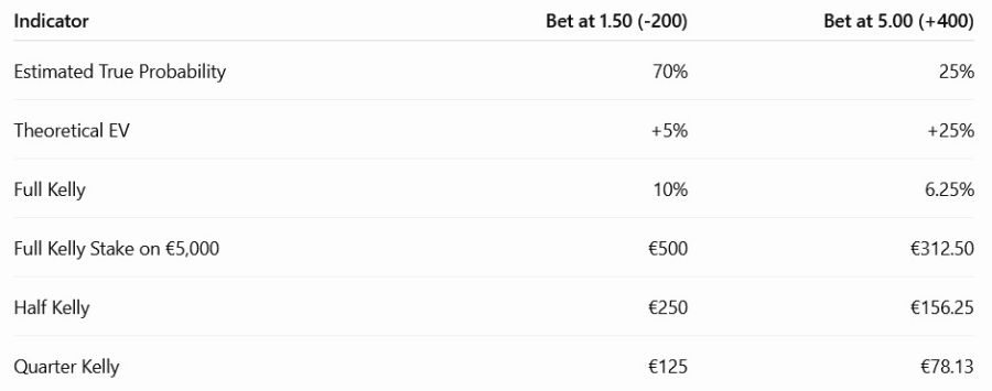
Amounts are rounded to the nearest cent.
This table illustrates an essential principle:
Edge and odds must be analyzed together.
The theoretical optimal Stake does not depend solely on the probability of winning or on expected ROI.
16. Why Full Kelly Can Be Too Aggressive
In the previous examples, the theoretical fractions may appear high.
However, they rely on a major assumption:
You know the true probability of each outcome accurately.
In sports betting, the true probability is generally not directly observable.
It must be estimated.
And an error of just a few percentage points can significantly change the calculation.
This is why applying Full Kelly without accounting for model uncertainty can lead to substantial Drawdowns.
Fractional Kelly reduces this exposure.
However, it does not eliminate Variance or the risk of estimation errors.
17. The Importance of Accurate Probability Estimates
Let's consider a selection at:
5.00 (+400)
You estimate its probability of winning at:
25%
Theoretical EV:
+25%
But suppose the actual probability is:
19%
The EV becomes:
(0.19 × 5.00 - 1) × 100 = -5%
A six-percentage-point difference in the probability estimate has transformed a supposedly attractive bet into an unfavorable one.
This is why identifying a large Edge is not enough.
You must also assess the reliability of your estimate.
18. Estimation Errors Can Be Particularly Costly
At high odds, a few percentage points of probability can represent a substantial difference in EV.
Consider odds of 5.00 (+400).
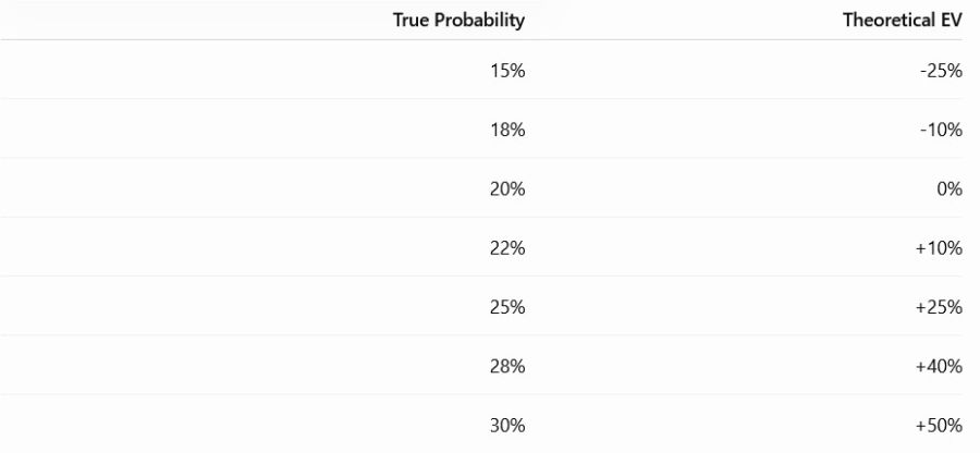
A strategy that appears extremely profitable can therefore become unprofitable if probabilities are estimated incorrectly.
This issue is not limited to high odds, but its impact can be particularly visible in these markets.
19. The Role of CLV in Evaluating a Strategy
At Bet2invest, Closing Line Value (CLV) is a particularly useful indicator.
It allows bettors to compare the odds obtained when a selection was made with the odds available at market closing.
Consider an example.
You obtain Pinnacle odds of:
5.00 (+400)
At closing, the odds have moved to:
4.50 (+350)
You obtained higher odds than the closing price.
This represents positive CLV when comparing the raw odds.
However:
Positive CLV does not guarantee a winning bet or definitively prove future profitability.
Nevertheless, it can help assess execution quality and the value of the prices obtained, particularly over a large Sample Size.
20. A Bet at 5.00 (+400) With Positive CLV May Be More Attractive Than One at 1.50 (-200)
Imagine two selections.
Selection A
Odds obtained:
1.50 (-200)
Closing odds:
1.55 (approximately -182)
You obtained lower odds than the closing price.
The raw CLV is negative.
Selection B
Odds obtained:
5.00 (+400)
Closing odds:
4.50 (+350)
You obtained higher odds than the closing price.
The raw CLV is positive.
Even though Selection B has a lower probability of winning, its price may be more attractive relative to the market.
This is an essential distinction:
Good odds are not necessarily low odds.
Good odds are odds that exceed the fair value you estimate for an event.
21. Higher Odds Require Greater Patience
With a strategy whose average odds are 5.00 (+400), wins may be relatively far apart.
Even if the model has a positive Edge, the bettor must accept extended periods without profit.
This requires:
- A sufficiently strong Bankroll.
- An appropriate Unit.
- Consistent discipline.
- A clear understanding of Variance.
- A substantial Sample Size for performance analysis.
The main danger would be changing Stakes emotionally after several losses.
22. Never Confuse Winning Frequency With Profitability
A strategy can achieve:
70% winning selections
and still lose money.
Another strategy can achieve:
25% winning selections
and remain profitable.
Everything depends on the odds obtained.
Example A
Average Odds:
1.40 (approximately -250)
Win Rate:
70%
Theoretical ROI:
(0.70 × 1.40 - 1) × 100 = -2%
Example B
Average Odds:
5.00 (+400)
Win Rate:
25%
Theoretical ROI:
+25%
The Win Rate alone is never sufficient to determine the quality of a strategy.
23. ROI Must Always Be Interpreted Alongside Sample Size
Suppose a Tipster reports:
ROI = +20%
over 50 bets.
This result may be interesting.
However, it does not carry the same statistical weight as an ROI of:
+8%
over 5,000 bets.
Sample Size is essential when evaluating the reliability of performance.
This is particularly important for high-odds strategies, whose results generally show greater dispersion.
Just a few wins can significantly change the observed ROI.
24. Why High-Odds Strategies Can Experience Large Drawdowns
Consider a strategy using:
1U = €50
If it experiences:
15 consecutive losses
the Drawdown associated with that sequence is:
-15U = -€750
On a €5,000 Bankroll, this represents:
-15%
Such a sequence can be compatible with a high-odds strategy, even one that is profitable over the long term.
This demonstrates that Unit size should also reflect the Variance profile of the strategy.
25. Should You Use a Smaller Unit for High-Odds Strategies?
In some cases, yes.
If a strategy has:
- A low winning frequency.
- High Variance.
- A history of substantial Drawdowns.
- Uncertain Edge estimates.
It may be appropriate to reduce the fraction of Bankroll staked on each bet.
For example:
0.50U instead of 1U
However, this decision should result from a risk analysis.
It should not be based on an automatic rule that every high-odds selection is a bad bet.
26. Example With a €5,000 Bankroll
Let's compare different Stake levels.

The odds do not change the amount lost when a bet fails.
The Stake determines that loss.
However, the probability of losing several consecutive bets depends on the profile of the selections.
27. The Same Unit Can Represent Different Risks Depending on the Strategy
Imagine two strategies.
Strategy A
Average Odds:
1.50 (-200)
True Win Probability:
70%
Strategy B
Average Odds:
5.00 (+400)
True Win Probability:
25%
Both use:
1U = €50
The maximum loss per bet is identical.
However, the distributions of results are different.
Strategy B will experience more individual losses on average, offset by larger profits when it wins.
Consequently, its Drawdown profile may be much more pronounced.
28. Risk of Ruin Depends on Several Variables
Risk of Ruin does not depend solely on Stake size.
It depends in particular on:
Bankroll size
Stake size
Winning probabilities
Odds
Actual Edge
Variance
Correlations between bets
and:
The time horizon considered.
Two strategies using exactly the same Unit can therefore have different risks of ruin.
29. Be Careful With Correlated Bets
So far, our examples have assumed independent bets.
But in reality, several selections may be related.
For example:
- Multiple bets on the same match.
- Multiple markets depending on the same match scenario.
- Several Tipsters using similar models.
- Multiple selections exposed to the same underlying event.
If several bets are strongly correlated, staking 1U on each does not necessarily mean that risk is properly diversified.
Stake Sizing must also account for the Bankroll's overall exposure.
30. Market Liquidity Can Influence Stake Size
In some markets, it is possible to place large bets without significantly affecting the price obtained.
In others, Liquidity is lower.
This is particularly relevant in:
Niche sports
Lower-division competitions
Specialized betting markets
A strategy may offer an attractive theoretical Edge but may not allow a large Stake to be executed at the desired odds.
This is why strategy quality should also be evaluated under actual market conditions.
31. Should Stakes Be Determined by Odds Ranges?
Some bettors use a table like this:
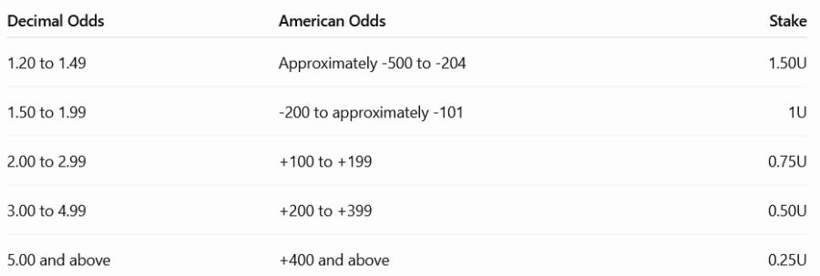
This table may appear cautious.
However, it has a major weakness:
It does not account for Edge.
Two bets at the same odds can have completely different Expected Values.
Similarly, a bet at 5.00 (+400) can have a higher Edge than a bet at 1.50 (-200).
Therefore, a table based solely on odds is not a mathematically optimal Stake Sizing method.
It may serve as a simplified risk-limiting rule, but not as proof of Stake optimization.
32. The Danger of Betting More on Favorites
Many bettors tend to stake more on favorites.
They consider low odds reassuring.
But favorites lose too.
And when Stakes are large, a single loss can erase several previous wins.
Consider odds of 1.50 (-200).
With a Stake of:
€100
Each win produces:
+€50
But each loss costs:
-€100
Therefore, two wins are needed to compensate for one loss, ignoring other considerations.
Low odds do not protect you from poor Stake Management.
33. The Opposite Danger: Betting Too Much on Underdogs
Conversely, some bettors are attracted by the potential profits offered by high odds.
Odds of 5.00 (+400) promise a substantial payout.
But staking an excessive proportion of Bankroll on low-probability outcomes can generate considerable Drawdowns.
High odds do not justify increasing Stakes either.
What matters remains:
The quality of the price obtained relative to the estimated true probability.
34. The Importance of Long-Term Discipline
Good Bankroll Management must remain applicable over:
100 bets
500 bets
1,000 bets
or more.
It should not depend on the emotions caused by the most recent result.
It must be robust enough to withstand:
- Losing Streaks.
- Drawdowns.
- Periods with low winning frequency.
- Estimation errors.
- Changes in market conditions.
The goal is not to optimize each individual bet at the cost of excessive risk.
It is to preserve your ability to exploit an Edge over time.
35. High-Odds Strategies Sometimes Require a Larger Bankroll
Suppose you want to limit Drawdowns to a level compatible with your risk tolerance.
If your strategy frequently experiences long Losing Streaks, you can:
Increase your Bankroll
or:
Reduce your Unit size.
Both solutions reduce the relative impact of losses on your capital.
However, they do not change the intrinsic quality of the selections.
Better Bankroll Management does not create an Edge.
It simply allows you to better withstand the risks associated with an assumed or demonstrated Edge.
36. How Should You Evaluate a Tipster Based on Average Odds?
When analyzing a Tipster's performance, it is useful to examine:
ROI
CLV
Sample Size
Average Odds
Win Rate
Maximum Drawdown
Flat Stakes Summary (1U)
Market Liquidity
These indicators should be interpreted together.
A Tipster whose average odds are 1.50 (-200) should not be evaluated in exactly the same way as one whose average odds are 5.00 (+400).
Their Variance profiles are different.
Their winning frequencies are different.
Their distributions of profits and losses are different.
37. Why Flat Stakes Summary (1U) Remains an Important Benchmark
The Flat Stakes Summary (1U) makes it possible to compare the results of different strategies using standardized Stakes.
Each bet represents one Unit.
This makes it possible to measure:
Profits in Units
ROI
Drawdowns
and:
Performance consistency
without mixing those results with personal Stake Sizing decisions.
This is particularly useful when comparing Tipsters with different average odds.
However, a complete comparison must always consider Variance and Sample Size.
38. Which Method Should an Experienced Bettor Prefer?
Several approaches can be reasonable.
Flat Betting
It offers simplicity, discipline, and transparency.
With:
1U = 1% of Bankroll
you clearly control the maximum loss on each bet.
Risk-Adjusted Flat Betting
You may use a smaller Unit for certain strategies with particularly high Variance.
For example:
0.50U
instead of:
1U
Such an adjustment should be based on objective criteria.
Fractional Kelly
If you have sufficiently reliable probability estimates, Fractional Kelly can provide a framework for adjusting Stakes according to Edge and odds.
However, caution is essential because of estimation errors.
None of these approaches guarantees profitability.
39. Our Example: Should You Bet €50 at 1.50 (-200) and €50 at 5.00 (+400)?
Let's return to our initial question.
Bankroll:
€5,000
Unit:
€50
Two bets:
1.50 (-200)
and:
5.00 (+400)
If you use strict Flat Betting, the answer is simple:
€50 on each bet.
However, if your objective is to adjust Stakes according to risk and Edge, you must examine:
- The estimated true probability of each selection.
- Expected Value.
- The reliability of those estimates.
- Expected Variance.
- Potential Drawdown.
- Correlations with your other bets.
- Your personal risk tolerance.
Odds alone cannot settle the question.
40. The 12 Mistakes to Avoid
- Believing that low odds automatically represent good value.
- Betting more on a favorite simply because it wins more often.
- Systematically reducing Stakes on high odds without analyzing Edge.
- Increasing Stakes on underdogs solely because of the potential payout.
- Confusing Win Rate with profitability.
- Ignoring Expected Value.
- Underestimating the Variance of high-odds strategies.
- Evaluating ROI without considering Sample Size.
- Applying Full Kelly with insufficiently reliable probability estimates.
- Ignoring correlations between bets.
- Changing Stakes after a Losing Streak to recover losses more quickly.
- Comparing Tipsters without considering their average odds and Drawdowns.
Conclusion
Should you bet the same amount at 1.50 (-200) and 5.00 (+400)?
There is no universal answer.
With strict Flat Betting, it is perfectly consistent to stake:
1U at 1.50 (-200)
and:
1U at 5.00 (+400)
This method standardizes Stakes and limits the maximum loss on each individual bet.
However, that does not mean both bets have the same statistical risk.
Odds of 5.00 (+400) generally imply a lower probability of winning and may lead to longer Losing Streaks.
Conversely, odds of 1.50 (-200) are not necessarily profitable.
The fundamental variable remains:
Edge.
And when attempting to optimize Stake size, you must also consider:
Estimated true probability
Odds
Variance
Model reliability
and:
Available Bankroll.
The Kelly Criterion demonstrates that a bet with a higher EV does not necessarily deserve a larger Stake.
For simple and disciplined Bankroll Management, Flat Betting remains a useful benchmark.
For more advanced management, adjustments based on Edge and risk may be considered.
But in every case:
Never choose your Stake simply because the odds appear low, high, reassuring, or spectacular.
Good Bankroll Management is not just about maximizing potential profits.
It is about protecting capital while allowing a genuine Edge to emerge over a sufficiently large Sample Size.
FAQ: Bankroll and Odds, Should You Bet the Same Amount at 1.50 (-200) and 5.00 (+400)?
Is a Bet at 1.50 (-200) Safer Than One at 5.00 (+400)?
It generally corresponds to a higher probability of winning. However, it is not necessarily more profitable. You must compare the odds offered with the estimated true probability.
Should You Always Bet Less on High Odds?
- Reducing Stakes can help control Variance, but the decision should also account for Edge and the reliability of its estimate.
Can You Stake 1U at All Odds?
Yes. This is the principle of Flat Betting. Each bet represents one Unit, regardless of its odds.
Can Odds of 5.00 (+400) Be More Profitable Than Odds of 1.50 (-200)?
Yes. Odds of 5.00 (+400) can offer a higher Expected Value if the true probability of winning is sufficiently high.
Why Do High Odds Produce Longer Losing Streaks?
Because they generally correspond to lower probabilities of winning. Losses are therefore more frequent, even though individual wins generate larger profits.
What Is the Break-Even Win Rate at 1.50 (-200)?
Approximately 66.67%.
What Is the Break-Even Win Rate at 5.00 (+400)?
Exactly 20%.
Does the Kelly Criterion Account for Odds?
Yes. It incorporates both the odds and the estimated probability of winning to calculate a theoretical fraction of Bankroll.
Should You Use Full Kelly?
Not necessarily. Full Kelly can be very aggressive, particularly when probability estimates are uncertain. Fractional Kelly can reduce exposure.
Can CLV Help Evaluate the Odds Obtained?
Yes. CLV compares the odds obtained with the closing odds. It is a useful indicator, but it does not guarantee that a bet or strategy will be profitable.
Does a High-Odds Strategy Require a Larger Bankroll?
It may require a larger Bankroll or a smaller Unit to withstand Drawdowns and extended Losing Streaks.
What Is the Most Important Rule?
Your Stake should follow a consistent risk management method, not simply the odds displayed. To go beyond Flat Betting, you must consider Edge, estimated true probability, and the reliability of that estimate.