In this article, you will learn about the reinterpretation of the different betting plans with Kelly's formula, as well as explanations of the impact on the loss and/or gain of units, the asymmetry of returns, and the symmetry of probability.

Four years ago, an article was published in the journal "Economics of Sport" on how a profitable bettor should bet under conditions where estimates of the true payoff probabilities are not available.

Whether a punter wishing to have consistent profitability over the long term should even be active in such conditions is debatable, but it turns out that many sports punters acknowledge that they are unable to estimate them accurately.

Nevertheless, their study is interesting in that it shows how different betting plans can be reinterpreted as variants of Kelly's criterion. In this article, I want to summarise their efforts and examine whether what they found can be improved.

Reinterpreting different betting plans with Kelly's formula

There is perhaps no more popular topic in the world of sports betting money management than the use of the Kelly criterion as a betting method. In particular, I have shown that for a simple Kelly bet, where only one bet at a time is placed before settlement, the strategy is able to take into account the risks associated with not knowing precisely your advantage on a bet-at-a-time basis, as long as you are accurate on average.

Loss per unit

The first of these strategies is the unit loss, or level stakes method, where the punter risks the same stake on each bet, regardless of the odds. The higher the odds, the greater the impact on the bankroll if the bet wins, but the lower the probability that the bet will win.

We can think of unit-loss betting as a Kelly plan in which the expected value or return is linearly proportional to the odds. Given that the size of the Kelly bet is given by EV / odds - 1 (where EV is the expected value, with anything greater than 0 being considered profitable), a unit-loss plan implies that this ratio remains constant.

For example, suppose the EV is 10% (0.1) and the odds are 2.00. The bet would be 0.1. If the odds increase to 4.00, this means that the EV must increase to 30% (0.3) for the stake to remain at 0.1. Odds of 101.00 would imply an EV of 10 or 1,000%, which seems a little unrealistic. This would imply real odds of only 9.18. Certainly no bookmaker would make such a serious mistake.

In fact, in the limit where the odds tend towards infinity, the real odds would tend towards a maximum value given by 1 / stake, in this case 10. One of the main criticisms levelled at unit-loss staking is that it places too great a risk on long-term bets with a low probability of winning. For the defenders of Kelly's criterion, this would only make sense if the EV actually increased in proportion to the odds, which, as we can see, is hardly credible.

Unit gain

The second money management plan generally used by punters is the unit bet. In this case, the stake is such that the punter aims to make the same profit whatever the odds. If the winning or profit target is €100, odds of 2.00 will require a stake of €100, while odds of 5.00 will require a stake of €25. The size of the stake is proportional to the reciprocal of the odds - 1.

In Kelly terms, the unit-win strategy implies that the EV is completely uncorrelated with the Kelly criterion; all EVs are the same whatever the odds.

As far as unit-loss betting is concerned, there's something not quite right. Is it possible for a bettor's advantage to be the same whether the odds are 1.11 or 111.00? The lessons learned from variance suggest that this is not very realistic. Indeed, if your EV for odds of 111.00 is 20% (0.2), the same EV for odds of 1.11 would imply that the true odds are less than 1, which is utter nonsense. Something cannot have a probability of outcome greater than 100%.

Impact of the unit

The authors have proposed an alternative staking plan: unit impact, on the assumption that this plan fits better with the Kelly staking method. The unit impact method keeps the bankroll difference between winning and losing constant, regardless of the length or brevity of the odds.

The unit impact stake is proportional to the reciprocal of the odds, unlike the unit win, which is the reciprocal of odds - 1. Thus, if the stake is €100 for odds of 2.00, the unit impact stake for odds of 5.00 will be €40. In each case, the difference between the win and the loss is €200 (+€100/€100 in the first case and +€160/€40 in the second).

For unit impact bets, the EV is proportional to the odds - 1 / odds. This means that the EV increases as the odds increase, but at a decreasing rate towards a limit, since this ratio tends rapidly towards 1. For example, if EV = 0.1 for a rating of 2.00, the EV limit will be 0.2. Although this scenario is not as extreme as for unit win betting, where the EV remains unchanged, it again seems to underestimate the possibility of higher EVs for longer odds.

Successful horse racing tipsters typically have returns well over double those focusing on the Asian handicap or point spread market, although this does not necessarily mean they are more skilled (or luckier); they simply have more variance on their side.

Following the author's lead, the table below illustrates how EV varies with odds for the three different betting plans, assuming EV = 3% for odds = 2.00 for each.

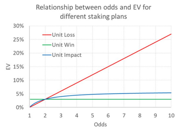
As discussed above, both the "unit loss" and "unit gain" betting schemes appear to imply unrealistic relationships between odds and EV.

The authors have analysed the betting picks database of a well-known prediction site and believe they have confirmed that the relationship between EV and the odds implied by the unit impact bet best reflects the observed and expected returns of the tipsters (the latter being based on closing prices). I am still not convinced. I repeat, the unit impact method will only ever produce an EV that is at most double the EV for odds = 2.00. Is there a better alternative?

Revisiting the T-distribution

Three years ago, I presented the use of the T-distribution to evaluate prognosticators and distinguish luck from skill. Similar to the normal distribution (and used in its place when we only know the standard deviation of the sample and not that of the population), it makes it possible to determine the degree of improbability of a given sample by assuming that the population mean is known.

I've used the T-distribution a lot in my work to help punters work out the probability of their outcomes being the result of chance, assuming they have no skill. The lower the probability, the more subjectively confident you can be that chance has nothing to do with your betting profits.

At the heart of this test is the t-statistic or t-score, from which probabilities can be derived. I have shown that for a unit-loss bet, and when the odds of your record do not vary too much, this statistic can be approximated with the following formula.

where n is the number of bets, o the average odds and r the return on investment or return + 1.

Like the z-score, which handicappers may be more familiar with, this is essentially a measure of the number of standard deviations your return deviates from an expected mean of zero, if you bet without skill and at fair odds. A t-score of 2, for example, means that a better return than your record is expected only 2.5% of the time, assuming you have no skills. The t-score is therefore a type of probability measure. The higher the t-score, the less likely the observation. Let's use it to determine the probability of different EVs (assuming no skills) based on the odds we are betting.

Asymmetric returns

Suppose you bet on a team with an 80% chance of winning, at odds of 1.25. Now let's suppose that the bookmaker wrongly thinks that the probability of winning is 75%. He is running a promotion and has no margin. His odds are 1.333. Your EV is therefore 6.667% (1.333/1.25 - 1 or 0.80/0.75 - 1).

Now consider a second scenario: the true chance is 20% (fair odds of 5.00), but the bookmaker reckons it is 15% (published odds of 6.667). This time, your EV is 33.33% (6.667/5.00 - 1 or 0.20/0.15 - 1). The difference in expected percentage gain between your estimate and that of the bookmaker is the same, but the EV is 5 times greater. It seems that in terms of EV, the higher the odds, the greater the penalty for equivalent errors. But what is the probability of these errors?

The symmetry of probability

Let's rewrite the t-score formula above (assuming that all our bets have the same odds, o). Since we know that r = q / p, where p is the implied probability of the bookmaker's odds (i.e. 1/o) and q is your estimated probability (which is 'true' if your prediction model is accurate), we can show that :

Let's assume that n, our number of bets, is equal to 100. For q = 0.8 and p = 0.75, t = 1.25. Similarly, for q = 0.2 and p = 0.15, t = 1.25 too. Assuming that the bookmaker, and not our model, is actually correct, such a t-score would correspond to a probability of outcome of 10.7% (using Excel's =TDIST function).

Out of 100 bets, we should get a return greater than 6.667% for odds of 1.333, or greater than 33.33% for odds of 6.667, or 10.7% of the time. Higher returns at higher odds are just as likely as lower returns at shorter odds, which is why race tipsters have the illusion that they are better than handicappers, or worse if they lose.

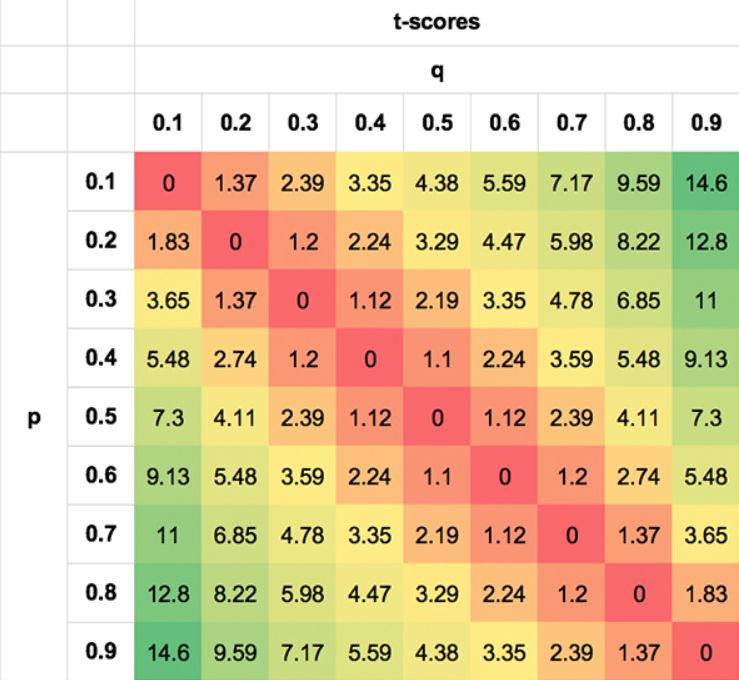
I have tried to illustrate this symmetry of probabilities using the following tables. The values are extreme simply to illustrate the point; obviously no punter will be able to do this well, or badly, for most scenarios.

The first shows the asymmetry of the EV for different pairs p, q. The second shows t-score symmetry. The second shows the symmetry of the t-scores. I have shown the absolute t-scores (removing the negative sign for negative EVs when q < p) for clarity. Not only is a p, q pair of 0.3/0.7 just as likely as a 0.7/0.3 pair, but so are pairs such as 0.7/0.5 and 0.3/0.1, 0.8/0.7 and 0.2/0.1 for the reasons described above.

A new EV dimension function

For a given odds and EV, there is a probability t (which doubles when the number of bets is multiplied by 4). We can rearrange the formula for the score t to express it in terms of r. This leads to a rather horrible quadratic with an even more horrible solution.

This is a much nastier solution than odds - 1 / odds, but let's plot it anyway for the scenario where EV = 0.03 and odds = 2.00. This graph is shown below, along with the previous EV functions for unit loss, unit gain and unit impact of the bet.

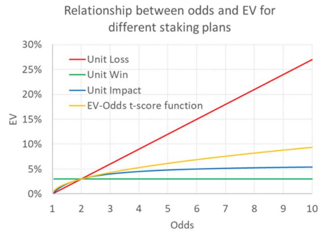
Although the function can be difficult to write, it is more intuitive because it interprets expected returns in terms of statistical probability. For unit-impact bets, the EV can never be more than 6% when it is 3% for odds of 2.00. But with my function, it can grow indefinitely, albeit not as unrealistically fast as for unit-loss betting, but in line with what statistical variance predicts. For odds of 10 it is 9.4%, for odds of 50 it is 23.3% and for odds of 1,000 it is 150%.

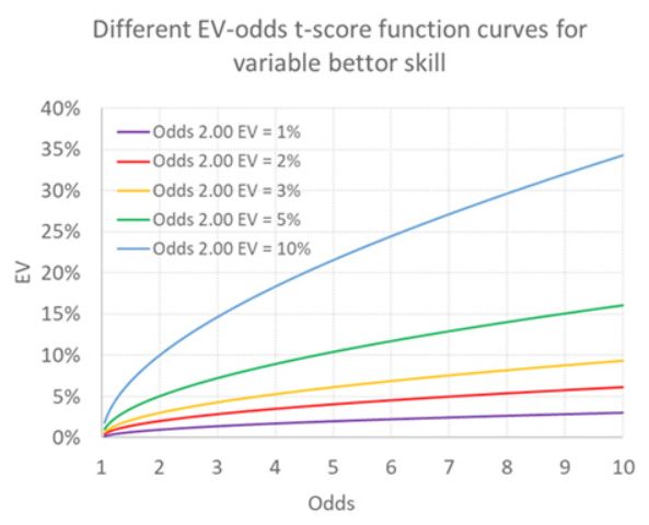
One obvious criticism is that this function, based on the T-score, assumes that the bettor has no skill. It simply expresses the probability of things happening assuming no skill is present. But this is a misinterpretation; even in the presence of skill, the same statistical laws associated with variance apply.

The position of the orange curve would change, but the shape would remain the same. I have illustrated below some possible trajectories for punters with varying degrees of luck or skill, depending on the term used. The initial curve for the punter with an EV of 3% at odds of 2.00 is always shown in orange.

Another criticism might be that we also assume that any skill is independent of the odds, i.e. that it is the same regardless of the odds. Given market inefficiencies, such as long-run bias, this assumption may not be appropriate.

Testing the function

Can we test the validity of this new EV- function? My betting system Wisdom of the Crowd, which those who follow me regularly on Twitter and Football-Data will be familiar with, uses Pinnacle's more efficient odds to estimate the EV available in other bookmakers' odds.

Using a sample of European domestic league match odds data dating back to the 2012/13 season, I found 55,237 occasions where a profitable EV (>0) was available. The average was 2.20% (for the record, the actual unit loss stakes performance was 1.77%, well within the model's statistical margins of error), with average odds of 3.30. With these figures, we can use my quadratic solution formula to construct an EV- function curve like the ones above. This is the orange curve below.

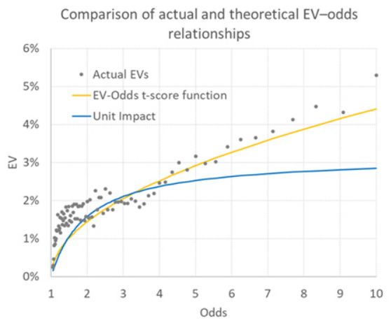
Compare this curve with the EVs of the actual model calculated on the basis of 1% payout expectations (shown as odds in the graph) and with the curve of the EV- function predicted by the unit impact bet. Although the match is not perfect, the EV t-score function is probably a better predictor of the approximate EVs based on the betting odds.

A reasoning

The more observant among you might now be thinking: what's the point of using an EV function to predict EV for different odds when your Wisdom of the Crowd model does this explicitly for each bet? This is indeed a valid judgement, and much of this article could therefore be considered rather theoretical.

Nevertheless, even accurate models (on average) have epistemic uncertainty for every bet. In addition, random (or inherent) uncertainty makes it virtually impossible to assess true payoff probabilities.

The aim of this exercise, as it was for the authors, was therefore to illustrate how you can try to approximate your EV when you recognise these quantitative uncertainties, when the prediction model does not explicitly estimate the probabilities of winning, or when the prediction method is more qualitative and based on intuition rather than data analysis. If you know your probabilities, this method will allow you to estimate your EV; if you know your EV, you can then determine the Kelly bet you should use.

This t-score methodology can be convoluted, but its results are derived from a more intuitive reasoning of the relationship between probability of win, expected value and probability of outcome, and by extension, how actual returns can be seen to vary with betting odds. For Kelly's followers, I think this method is more effective than unit impact staking, and certainly more effective than unit loss and unit gain.